Sliderule data I/O#
This notebook will highlight analyzing various coincident elevation measurements. We will find regions with and use slideruleearth.io service to retrieve ICESat-2 and GEDI point elevation measurements.
Note
Keep in mind, these measurements are from different sensor types, close in time, but not at exactly the same time. All measurements also have uncertainties, so we do not expect perfect agreement.
import coincident
from mpl_toolkits.axes_grid1.inset_locator import inset_axes
import matplotlib.pyplot as plt
import numpy as np

# For testing OR if you have access to a private cluster set that here
# https://slideruleearth.io/web/rtd/developer_guide/articles/private_clusters.html#private-clusters
# sliderule.init(verbose=True, organization="uw", desired_nodes=5, bypass_dns=True, time_to_live=60)
/home/docs/checkouts/readthedocs.org/user_builds/coincident/checkouts/latest/src/coincident/io/download.py:25: TqdmExperimentalWarning: Using `tqdm.autonotebook.tqdm` in notebook mode. Use `tqdm.tqdm` instead to force console mode (e.g. in jupyter console)
  from tqdm.autonotebook import tqdm
%matplotlib inline
# %config InlineBackend.figure_format = 'retina'
Identify a primary dataset#
Start by loading a full resolution polygon of a 3DEP LiDAR workunit which has a known start_datetime and end_datatime:
workunit = "CO_WestCentral_2019"
df_wesm = coincident.search.wesm.read_wesm_csv()
gf_lidar = coincident.search.wesm.load_by_fid(
    df_wesm[df_wesm.workunit == workunit].index
)
gf_lidar
| workunit | workunit_id | project | project_id | start_datetime | end_datetime | ql | spec | p_method | dem_gsd_meters | ... | seamless_category | seamless_reason | lpc_link | sourcedem_link | metadata_link | geometry | collection | datetime | dayofyear | duration | |
|---|---|---|---|---|---|---|---|---|---|---|---|---|---|---|---|---|---|---|---|---|---|
| 0 | CO_WestCentral_2019 | 175984 | CO_WestCentral_2019_A19 | 175987 | 2019-08-21 | 2019-09-19 | QL 2 | USGS Lidar Base Specification 1.3 | linear-mode lidar | 1.0 | ... | Meets | Meets 3DEP seamless DEM requirements | https://rockyweb.usgs.gov/vdelivery/Datasets/S... | https://prd-tnm.s3.amazonaws.com/index.html?pr... | https://prd-tnm.s3.amazonaws.com/index.html?pr... | MULTIPOLYGON (((-106.13571 38.4146, -106.1702 ... | 3DEP | 2019-09-04 12:00:00 | 247 | 29 |
1 rows × 33 columns
Search secondary datasets#
Provide a list that will be searched in order. The list contains tuples of dataset aliases and the temporal pad in days to search before the primary dataset start and end dates
secondary_datasets = [
    ("gedi", 40),  # +/- 40 days from lidar
    ("icesat-2", 60),  # +/- 60 days from lidar
]

gf_gedi, gf_is2 = coincident.search.cascading_search(
    gf_lidar,
    secondary_datasets,
    min_overlap_area=30,  # km^2
)
Get ICESat-2 ATL06 Data#
We’ve identified 7 granules of icesat-2 data to examine, but there is no need to work with the entire granule, which spans a huge geographic extent. Instead we’ll retrieve a subset of elevation values in the area of interest for each granule.
# Hone in on single granule as a pandas series
i = 0
granule_gdf = gf_is2.iloc[[i]]
granule = gf_is2.iloc[i]
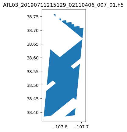
granule_gdf.plot() # needs to be a geodataframe
plt.title(granule.id);
# The icesat-2 track trends N-S, and is crossed by multiple GEDI tracks, resulting in the crosshatched appearance
data_atl08 = coincident.io.sliderule.subset_atl08(
    granule_gdf,
    include_worldcover=True,
)
print(len(data_atl08))
data_atl08.iloc[0]
43
n_te_photons                                                           14
segment_snowcover                                                       1
region                                                                  6
gt                                                                     20
h_te_uncertainty                                               156.686874
solar_elevation                                                 52.006374
segment_id_beg                                                     787276
canopy_h_metrics        [0.6411133, 2.3569336, 2.4990234, 3.6000977, 4...
segment_cover                                                          14
worldcover.time_ns                        [2021-06-30T00:00:00.000000000]
terrain_slope                                                    0.071977
rgt                                                                   211
h_te_median                                                   2193.446289
h_canopy                                                        17.465576
n_ca_photons                                                           14
worldcover.fileid                                                     [0]
h_mean_canopy                                                    7.781447
spot                                                                    2
worldcover.value                                                Grassland
n_seg_ph                                                               51
h_canopy_uncertainty                                            148.38472
h_max_canopy                                                    17.465576
h_min_canopy                                                     0.538574
srcid                                                                   3
segment_landcover                                                      30
cycle                                                                   4
canopy_openness                                                  5.101137
geometry                   POINT (-107.73307800292969 38.657413482666016)
Name: 2019-07-11 21:56:57.789710080, dtype: object
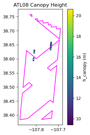
# Plot this data and overlay footprint
fig, ax = plt.subplots(figsize=(4, 5))
plt.scatter(
    x=data_atl08.geometry.x,
    y=data_atl08.geometry.y,
    c=data_atl08.h_canopy,
    s=10,
)
granule_gdf.dissolve().boundary.plot(ax=ax, color="magenta")
cb = plt.colorbar()
ax.set_title("ATL08 Canopy Height")
cb.set_label("h_canopy (m)")
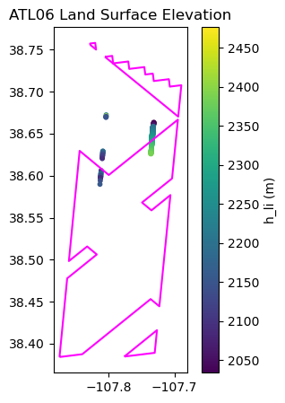
# ATL06 corresponds to land surface elevation
data_is2 = coincident.io.sliderule.subset_atl06(
    granule_gdf,
    include_worldcover=True,
)
print(len(data_is2))
data_is2.iloc[0]
284
tide_ocean                                                          NaN
region                                                                6
gt                                                                   50
n_fit_photons                                                        17
w_surface_window_final                                         4.128994
atl06_quality_summary                                                 0
worldcover.time_ns                      [2021-06-30T00:00:00.000000000]
rgt                                                                 211
r_eff                                                           0.02509
seg_azimuth                                                 -174.518005
bsnow_h                                                             NaN
h_robust_sprd                                                  0.688166
sigma_geo_h                                                    5.002733
worldcover.fileid                                                   [0]
h_li_sigma                                                     0.467223
dh_fit_dx                                                       0.01674
x_atc                                                   15767759.895834
spot                                                                  5
y_atc                                                       4675.225098
worldcover.value                                             Tree cover
srcid                                                                 3
bsnow_conf                                                          127
cycle                                                                 4
h_li                                                        2245.366943
segment_id                                                       787226
geometry                  POINT (-107.80409390031208 38.67234499367456)
Name: 2019-07-11 21:56:57.269883392, dtype: object
# Plot this data and overlay footprint
fig, ax = plt.subplots(figsize=(4, 5))
plt.scatter(
    x=data_is2.geometry.x,
    y=data_is2.geometry.y,
    c=data_is2.h_li,
    s=10,
)
granule_gdf.dissolve().boundary.plot(ax=ax, color="magenta")
cb = plt.colorbar()
ax.set_title("ATL06 Land Surface Elevation")
cb.set_label("h_li (m)")
Note
sliderule gets data from the envelope of multipolygon, not only data within intersecting GEDI tracks. Along-track gaps are where there is missing data.
Spatial join: nearest points#
NOTE: we will not worry about the difference in time of acquisition between adjacent points for now
def get_nearest_points(gf_reference, gf_compare, max_distance=100):
"""Get nearest points across two geodataframes within a maximum distance in meters.
NOTE: reprojects dataframes to UTM and returns dataframe point in UTM
"""
gf_left_utm = gf_reference.to_crs(gf_reference.estimate_utm_crs())
gf_right_utm = gf_compare.to_crs(gf_compare.estimate_utm_crs())
nearest_points = gf_left_utm.sjoin_nearest(
gf_right_utm,
how="left",
max_distance=max_distance,
distance_col="distances",
)
return nearest_points
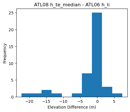
# ATL08 has h_te_median as an estimate of median terrain elevation.
# ATL06 has h_li as the land surface elevation which we expect to be close but not exactly the same
# based on algorithm differences and point spacing.
nearest_points = get_nearest_points(data_atl08, data_is2, max_distance=100)
nearest_points.head()
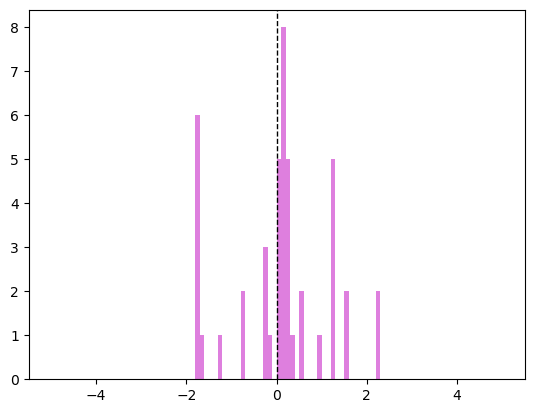
fig, ax = plt.subplots(figsize=(5, 4))
(nearest_points["h_te_median"] - nearest_points["h_li"]).plot.hist(bins=10, ax=ax)
plt.title("ATL08 h_te_median - ATL06 h_li")
plt.xlabel("Elevation Difference (m)");
Get GEDI Data#
# Here, we specify aoi=granule_gdf to only return GEDI data
# in our icesat-2 track of interest
data_gedi = coincident.io.sliderule.subset_gedi02a(
    gf_gedi,
    aoi=granule_gdf,
    include_worldcover=True,
)
data_gedi.head(2)
| orbit | track | elevation_lm | solar_elevation | shot_number | flags | worldcover.time_ns | worldcover.fileid | elevation_hr | worldcover.value | beam | sensitivity | srcid | geometry | |
|---|---|---|---|---|---|---|---|---|---|---|---|---|---|---|
| time_ns | ||||||||||||||
| 2019-08-20 14:38:24.715338496 | 3893 | 583 | 1747.265747 | 23.696064 | 38930000200401008 | 130 | [2021-06-30T00:00:00.000000000] | [25769803776] | 1750.487671 | Grassland | 0 | 0.901893 | 121 | POINT (-107.87052 38.49553) |
| 2019-08-20 14:38:24.723602432 | 3893 | 583 | 1747.438110 | 23.696466 | 38930000200401009 | 130 | [2021-06-30T00:00:00.000000000] | [25769803776] | 1750.847290 | Grassland | 0 | 0.901397 | 121 | POINT (-107.87001 38.49585) |
# Plot this data and overlay footprint
fig, ax = plt.subplots(figsize=(4, 5))
plt.scatter(
    x=data_gedi.geometry.x,
    y=data_gedi.geometry.y,
    c=data_gedi.elevation_hr,
    s=10,
)
granule_gdf.dissolve().boundary.plot(ax=ax, color="magenta")
cb = plt.colorbar()
cb.set_label("elevation_hr (m)")
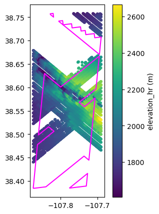
NOTE Like ICESat-2, it’s possible to have points falling outside the estimated footprints
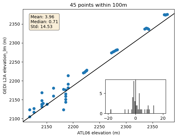
# find nearest IS2 point to each GEDI
close_gedi = get_nearest_points(data_gedi, data_is2, max_distance=100)
close_gedi = close_gedi[close_gedi["distances"].notna()]
fig, ax = plt.subplots()
plt.scatter(close_gedi.h_li, close_gedi.elevation_lm)
ax.axline((0, 0), slope=1, color="k", transform=ax.transAxes)
plt.xlabel("ATL06 elevation (m)")
plt.ylabel("GEDI L2A elevation_lm (m)")
plt.title(f"{len(close_gedi)} points within 100m")


# Add statistics and inset histogram to plot
inset_ax = inset_axes(ax, width="40%", height="30%", borderpad=2, loc="lower right")


residuals = close_gedi.h_li - close_gedi.elevation_lm
mean_residual = np.mean(residuals)
median_residual = np.median(residuals)
std_residual = np.std(residuals)
textstr = "\n".join(
    (
        f"Mean: {mean_residual:.2f}",
        f"Median: {median_residual:.2f}",
        f"Std: {std_residual:.2f}",
    )
)
props = dict(boxstyle="round", facecolor="wheat", alpha=0.5)
ax.text(
    0.05,
    0.95,
    textstr,
    transform=ax.transAxes,
    fontsize=10,
    verticalalignment="top",
    bbox=props,
)

_ = inset_ax.hist(residuals, bins=50, range=(-20, 20), color="gray")
inset_ax.axvline(0, color="k", linestyle="-", linewidth=1);
Sample 3DEP#
Sample 3DEP 1m DEM at the subset of GEDI Points
# Warning: this relies on TNM API, which is often down :(
close_gedi_3dep = coincident.io.sliderule.sample_raster(
    close_gedi.to_crs(4326),  # reproject to lat/lon for sampling
    asset_key="usgs3dep-1meter-dem",
    # Restrict to only DEMs derived from specific WESM LiDAR project
    project_name=gf_lidar["project"].iloc[0],
)
---------------------------------------------------------------------------
FatalError                                Traceback (most recent call last)
Cell In[16], line 2
      1 # Warning: this relies on TNM API, which is often down :(
----> 2 close_gedi_3dep = coincident.io.sliderule.sample_raster(
      3     close_gedi.to_crs(4326),  # reproject to lat/lon for sampling
      4     asset_key="usgs3dep-1meter-dem",
      5     # Restrict to only DEMs derived from specific WESM LiDAR project

File ~/checkouts/readthedocs.org/user_builds/coincident/checkouts/latest/src/coincident/_utils.py:29, in depends_on_optional.<locals>.decorator.<locals>.wrapper(*args, **kwargs)
     25     message = (
     26         f"Optional dependency {module_name} not found ({func.__name__})."
     27     )
     28     raise ImportError(message)
---> 29 return func(*args, **kwargs)

File ~/checkouts/readthedocs.org/user_builds/coincident/checkouts/latest/src/coincident/io/sliderule.py:401, in sample_raster(gf, asset_key, project_name)
    399 else:
    400     poly = _gdf_to_sliderule_polygon(gfll)
--> 401     geojson = earthdata.tnm(
    402         short_name="Digital Elevation Model (DEM) 1 meter", polygon=poly
    403     )
    405     gfsr = raster.sample(asset_key, points, {"catalog": geojson})
    407     if project_name is not None:
    408         # Allow NaNs if restricting to a single WESM project

File ~/checkouts/readthedocs.org/user_builds/coincident/checkouts/latest/.pixi/envs/docs/lib/python3.14/site-packages/sliderule/earthdata.py:306, in tnm(short_name, polygon, time_start, time_end, as_str)
    295 parms = {
    296     k: v for k, v in {
    297     "api": "tnm",
   (...)    302     "max_resources": MaxRequestedResources
    303 }.items() if v is not None}
    305 # Make Request
--> 306 geojson = sliderule.source("earthdata", parms, rethrow=True)
    308 # Return GeoJSON
    309 if as_str:

File ~/checkouts/readthedocs.org/user_builds/coincident/checkouts/latest/.pixi/envs/docs/lib/python3.14/site-packages/sliderule/sliderule.py:205, in source(api, parm, stream, callbacks, path, session, rethrow, sign)
    166 '''
    167 Perform API call to SlideRule service
    168
   (...)    202     {'time': 1300556199523.0, 'format': 'GPS'}
    203 '''
    204 session = checksession(session)
--> 205 return session.source(api, parm=parm, stream=stream, callbacks=callbacks, path=path, rethrow=rethrow, sign=sign)

File ~/checkouts/readthedocs.org/user_builds/coincident/checkouts/latest/.pixi/envs/docs/lib/python3.14/site-packages/sliderule/session.py:307, in Session.source(self, api, parm, stream, callbacks, path, retries, rethrow, sign, headers)
    305 if not complete:
    306     if self.throw_exceptions or rethrow:
--> 307         raise FatalError(f'error in request to {url}: {rsps}')
    308     else:
    309         self.logger.error(f'Error in request to {url}: {rsps}')

FatalError: error in request to https://sliderule.slideruleearth.io/source/earthdata: HTTP error <500> {'code': -4, 'error': '{"error": "Expecting value: line 1 column 1 (char 0)", "showToast": true, "toastMessage": "Expecting value: line 1 column 1 (char 0)", "toastType": "warning"}'}
# Add 3DEP elevation values to existing dataframe
close_gedi["elevation_3dep"] = close_gedi_3dep.value.values
---------------------------------------------------------------------------
NameError                                 Traceback (most recent call last)
Cell In[17], line 2
      1 # Add 3DEP elevation values to existing dataframe
----> 2 close_gedi["elevation_3dep"] = close_gedi_3dep.value.values

NameError: name 'close_gedi_3dep' is not defined
# Geometries of nearest IS2 points
close_is2 = data_is2.loc[close_gedi.time_ns_right]
# Sample 3DEP at the subset of GEDI Points
close_is2_3dep = coincident.io.sliderule.sample_raster(
    close_is2,
    asset_key="usgs3dep-1meter-dem",
    project_name=gf_lidar["project"].iloc[0],
)
/home/docs/checkouts/readthedocs.org/user_builds/coincident/checkouts/latest/.pixi/envs/docs/lib/python3.14/site-packages/geopandas/array.py:411: UserWarning: Geometry is in a geographic CRS. Results from 'sjoin_nearest' are likely incorrect. Use 'GeoSeries.to_crs()' to re-project geometries to a projected CRS before this operation.

  warnings.warn(
close_is2["elevation_3dep"] = close_is2_3dep.value.values
plt.axvline(0, color="k", linestyle="dashed", linewidth=1)

diff_3dep = close_is2.h_li.values - close_is2.elevation_3dep
label = f"ICESat-2 (median={np.nanmedian(diff_3dep):.2f}, mean={np.nanmean(diff_3dep):.2f}, std={np.nanstd(diff_3dep):.2f}, n={len(diff_3dep)})"
plt.hist(diff_3dep, range=[-5, 5], bins=100, color="m", alpha=0.5, label=label)

diff_3dep = close_gedi.elevation_lm.values - close_gedi.elevation_3dep
label = f"GEDI2A (median={np.nanmedian(diff_3dep):.2f}, mean={np.nanmean(diff_3dep):.2f}, std={np.nanstd(diff_3dep):.2f}, n={len(diff_3dep)})"
plt.hist(diff_3dep, range=[-5, 5], bins=100, color="c", alpha=0.5, label=label)

plt.xlabel("elevation difference (m)")
plt.title("Altimeter Elevation - 3DEP 1m DEM")
plt.xlim(-5, 5)
plt.legend(loc="upper left");
---------------------------------------------------------------------------
AttributeError                            Traceback (most recent call last)
Cell In[21], line 7
      3 diff_3dep = close_is2.h_li.values - close_is2.elevation_3dep
      4 label = f"ICESat-2 (median={np.nanmedian(diff_3dep):.2f}, mean={np.nanmean(diff_3dep):.2f}, std={np.nanstd(diff_3dep):.2f}, n={len(diff_3dep)})"
      5 plt.hist(diff_3dep, range=[-5, 5], bins=100, color="m", alpha=0.5, label=label)
      6
----> 7 diff_3dep = close_gedi.elevation_lm.values - close_gedi.elevation_3dep
      8 label = f"GEDI2A (median={np.nanmedian(diff_3dep):.2f}, mean={np.nanmean(diff_3dep):.2f}, std={np.nanstd(diff_3dep):.2f}, n={len(diff_3dep)})"
      9 plt.hist(diff_3dep, range=[-5, 5], bins=100, color="c", alpha=0.5, label=label)
     10

File ~/checkouts/readthedocs.org/user_builds/coincident/checkouts/latest/.pixi/envs/docs/lib/python3.14/site-packages/pandas/core/generic.py:6206, in NDFrame.__getattr__(self, name)
   6202             and name not in self._accessors
   6203             and self._info_axis._can_hold_identifiers_and_holds_name(name)
   6204         ):
   6205             return self[name]
-> 6206         return object.__getattribute__(self, name)

AttributeError: 'GeoDataFrame' object has no attribute 'elevation_3dep'