Comparing Elevation Measurements#
Once you have an area of interest with multiple overlapping DEMs and/or laser altimetry measurements, you can quickly compare elevation values. coincident supports a main plotting panel for elevation comparisons, as well as dynamic boxplots and histograms for elevation differences over various terrain characteristics and land cover types.
This notebook highlights the following functions:
coincident.plot.compare_dems
coincident.plot.boxplot_slope
coincident.plot.boxplot_elevation
coincident.plot.boxplot_aspect
coincident.plot.hist_esa
Warning
Plotting routines are currently only tested for comparing datasets in EPSG:7912 (ITRF 2014)
import coincident
import geopandas as gpd
from shapely.geometry import box
import rioxarray as rxr
import xarray as xr
import xdem
import numpy as np
import matplotlib.pyplot as plt
from rasterio.enums import Resampling

%matplotlib inline
Load reference DEM#
workunit = "CO_WestCentral_2019"
df_wesm = coincident.search.wesm.read_wesm_csv()
gf_lidar = coincident.search.wesm.load_by_fid(
    df_wesm[df_wesm.workunit == workunit].index
)

gf_lidar
| workunit | workunit_id | project | project_id | start_datetime | end_datetime | ql | spec | p_method | dem_gsd_meters | ... | seamless_category | seamless_reason | lpc_link | sourcedem_link | metadata_link | geometry | collection | datetime | dayofyear | duration | |
|---|---|---|---|---|---|---|---|---|---|---|---|---|---|---|---|---|---|---|---|---|---|
| 0 | CO_WestCentral_2019 | 175984 | CO_WestCentral_2019_A19 | 175987 | 2019-08-21 | 2019-09-19 | QL 2 | USGS Lidar Base Specification 1.3 | linear-mode lidar | 1.0 | ... | Meets | Meets 3DEP seamless DEM requirements | https://rockyweb.usgs.gov/vdelivery/Datasets/S... | http://prd-tnm.s3.amazonaws.com/index.html?pre... | http://prd-tnm.s3.amazonaws.com/index.html?pre... | MULTIPOLYGON (((-106.13571 38.4146, -106.1702 ... | 3DEP | 2019-09-04 12:00:00 | 247 | 29 |
1 rows × 33 columns
# We will examine the 'sourcedem' 1m
# NOTE: it's important to note the *vertical* CRS of the data
gf_lidar.iloc[0]
workunit                                            CO_WestCentral_2019
workunit_id                                                      175984
project                                         CO_WestCentral_2019_A19
project_id                                                       175987
start_datetime                                      2019-08-21 00:00:00
end_datetime                                        2019-09-19 00:00:00
ql                                                                 QL 2
spec                                  USGS Lidar Base Specification 1.3
p_method                                              linear-mode lidar
dem_gsd_meters                                                      1.0
horiz_crs                                                          6350
vert_crs                                                           5703
geoid                                                          GEOID12B
lpc_pub_date                                        2021-01-30 00:00:00
lpc_update                                                          NaT
lpc_category                                                      Meets
lpc_reason                                  Meets 3DEP LPC requirements
sourcedem_pub_date                                  2021-01-29 00:00:00
sourcedem_update                                                    NaT
sourcedem_category                                                Meets
sourcedem_reason                     Meets 3DEP source DEM requirements
onemeter_category                                                 Meets
onemeter_reason                         Meets 3DEP 1-m DEM requirements
seamless_category                                                 Meets
seamless_reason                    Meets 3DEP seamless DEM requirements
lpc_link              https://rockyweb.usgs.gov/vdelivery/Datasets/S...
sourcedem_link        http://prd-tnm.s3.amazonaws.com/index.html?pre...
metadata_link         http://prd-tnm.s3.amazonaws.com/index.html?pre...
geometry              MULTIPOLYGON (((-106.1357105581 38.4146013052,...
collection                                                         3DEP
datetime                                            2019-09-04 12:00:00
dayofyear                                                           247
duration                                                             29
Name: 0, dtype: object
# NOTE: since we're going to compare to satellite altimetry, let's convert first to EPSG:7912 !
# GDAL / PROJ will use the following transform by default
!projinfo -s EPSG:6350+5703 -t EPSG:7912 -q -o proj
+proj=pipeline
  +step +inv +proj=aea +lat_0=23 +lon_0=-96 +lat_1=29.5 +lat_2=45.5 +x_0=0 +y_0=0
        +ellps=GRS80
  +step +proj=vgridshift +grids=us_noaa_g2018u0.tif +multiplier=1
  +step +proj=cart +ellps=GRS80
  +step +inv +proj=helmert +x=1.0053 +y=-1.90921 +z=-0.54157 +rx=0.02678138
        +ry=-0.00042027 +rz=0.01093206 +s=0.00036891 +dx=0.00079 +dy=-0.0006
        +dz=-0.00144 +drx=6.667e-05 +dry=-0.00075744 +drz=-5.133e-05
        +ds=-7.201e-05 +t_epoch=2010 +convention=coordinate_frame
  +step +inv +proj=cart +ellps=GRS80
  +step +proj=unitconvert +xy_in=rad +xy_out=deg
  +step +proj=axisswap +order=2,1
Now, let’s grab the vendor DEM products for two arbitrary tiles of this flight to look at elevation differences between the aerial LIDAR derved DEM, Copernicus GLO-30 DEM, ICESat-2 elevations, and GEDI elevations.
# We will rely on GDAL to do this reprojection
# gdalvsi = "/vsicurl?empty_dir=yes&url="
gdalvsi = "/vsicurl/"
url_tile_1 = f"{gdalvsi}https://prd-tnm.s3.amazonaws.com/StagedProducts/Elevation/OPR/Projects/CO_WestCentral_2019_A19/CO_WestCentral_2019/TIFF/USGS_OPR_CO_WestCentral_2019_A19_be_w1032n1780.tif"
url_tile_2 = f"{gdalvsi}https://prd-tnm.s3.amazonaws.com/StagedProducts/Elevation/OPR/Projects/CO_WestCentral_2019_A19/CO_WestCentral_2019/TIFF/USGS_OPR_CO_WestCentral_2019_A19_be_w1032n1779.tif"

# First build a mosaic in native 3D CRS
!gdalbuildvrt -q -a_srs EPSG:6350+5703 /tmp/mosaic.vrt '{url_tile_1}' '{url_tile_2}'
# Then reproject
!GDAL_DISABLE_READDIR_ON_OPEN=EMPTY_DIR gdalwarp -q -overwrite -t_srs EPSG:7912 -r bilinear /tmp/mosaic.vrt /tmp/mosaic_7912.tif
# Open our 'reference' DEM
da_lidar = rxr.open_rasterio("/tmp/mosaic_7912.tif", masked=True).squeeze()
da_lidar
<xarray.DataArray (y: 1917, x: 1465)> Size: 11MB
[2808405 values with dtype=float32]
Coordinates:
    band         int64 8B 1
  * x            (x) float64 12kB -108.0 -108.0 -108.0 ... -108.0 -108.0 -108.0
  * y            (y) float64 15kB 38.47 38.47 38.47 38.47 ... 38.46 38.46 38.46
    spatial_ref  int64 8B 0
Attributes:
    AREA_OR_POINT:  Area
    scale_factor:   1.0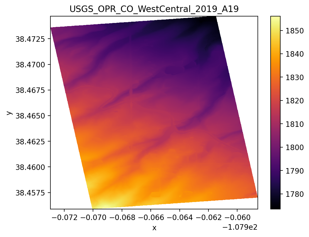
add_offset: 0.0# Plot a single DEM
ax = coincident.plot.plot_dem(da_lidar, title="USGS_OPR_CO_WestCentral_2019_A19");
Load secondary DEMs#
Note
Currently coincident facilitates loading select global DEMs in EPSG:7912, if your dataset is not in that CRS be sure to first reproject your data
# search geodataframe to grab the COP30 DEM
bbox_tile = da_lidar.rio.bounds()
poly_tile = box(*bbox_tile)
gf_tile = gpd.GeoDataFrame(geometry=[poly_tile], crs=da_lidar.rio.crs)
# NOTE: this is 30m data, but we are going to resample it to 1m to match our lidar
da_cop = coincident.io.xarray.load_dem_7912("cop30", aoi=gf_tile)
da_cop
<xarray.DataArray 'band_data' (y: 69, x: 53)> Size: 15kB
array([[1800.7252, 1800.2207, 1799.4016, ..., 1773.1454, 1770.5667,
        1770.0399],
       [1800.5754, 1799.8733, 1799.3422, ..., 1774.0353, 1771.1886,
        1770.74  ],
       [1800.5575, 1799.7347, 1799.4817, ..., 1772.8221, 1772.1632,
        1771.3894],
       ...,
       [1859.3857, 1858.9048, 1857.8425, ..., 1829.5653, 1828.9321,
        1828.7308],
       [1861.8115, 1861.497 , 1860.04  , ..., 1829.9324, 1830.4056,
        1830.1598],
       [1863.0483, 1862.5264, 1860.8612, ..., 1830.5692, 1830.6556,
        1830.5651]], dtype=float32)
Coordinates:
    band         int64 8B 1
  * x            (x) float64 424B -108.0 -108.0 -108.0 ... -108.0 -108.0 -108.0
  * y            (y) float64 552B 38.47 38.47 38.47 38.47 ... 38.46 38.46 38.46
    spatial_ref  int64 8B 0
Attributes:
AREA_OR_POINT: Pointds_cop_r = (
da_cop.rio.reproject_match(
da_lidar,
resampling=Resampling.bilinear,
)
.where(da_lidar.notnull())
.to_dataset(name="elevation")
)
ds_cop_r
<xarray.Dataset> Size: 11MB
Dimensions:      (x: 1465, y: 1917)
Coordinates:
    band         int64 8B 1
    spatial_ref  int64 8B 0
  * x            (x) float64 12kB -108.0 -108.0 -108.0 ... -108.0 -108.0 -108.0
  * y            (y) float64 15kB 38.47 38.47 38.47 38.47 ... 38.46 38.46 38.46
Data variables:
elevation (y, x) float32 11MB nan nan nan nan nan ... nan nan nan nan nan# Create hillshade variables for plot backgrounds
# This function expects Datasets
ds_lidar = da_lidar.to_dataset(name="elevation")
ds_lidar["hillshade"] = coincident.plot.hillshade(ds_lidar.elevation)
ds_cop_r["hillshade"] = coincident.plot.hillshade(ds_cop_r.elevation)
/home/docs/checkouts/readthedocs.org/user_builds/coincident/checkouts/v0.2/src/coincident/plot/utils.py:102: RuntimeWarning: invalid value encountered in cast
  return da.dims, data.astype(np.uint8)
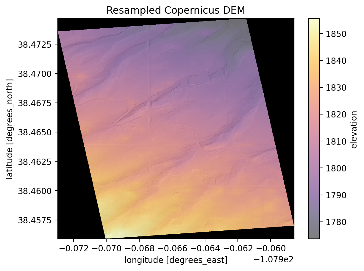
# Plot a single DEM with hillshade
ax = coincident.plot.plot_dem(
    ds_cop_r["elevation"],
    title="Resampled Copernicus DEM",
    da_hillshade=ds_lidar["hillshade"],
)
# Get GEDI
gf_gedi = coincident.search.search(
    dataset="gedi",
    intersects=gf_tile,
)
data_gedi = coincident.io.sliderule.subset_gedi02a(
    gf_gedi, gf_tile, include_worldcover=True
)
# Get ICESAT-2
gf_is2 = coincident.search.search(
    dataset="icesat-2",
    intersects=gf_tile,
)
data_is2 = coincident.io.sliderule.subset_atl06(
    gf_is2, gf_tile, include_worldcover=True
)
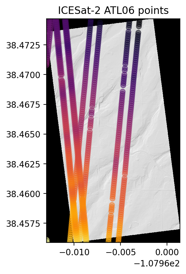
# NOTE: this works because ICESat-2 and GEDI are EPSG:7912
coincident.plot.plot_altimeter_points(
    data_is2, "h_li", da_hillshade=ds_lidar["hillshade"], title="ICESat-2 ATL06 points"
);
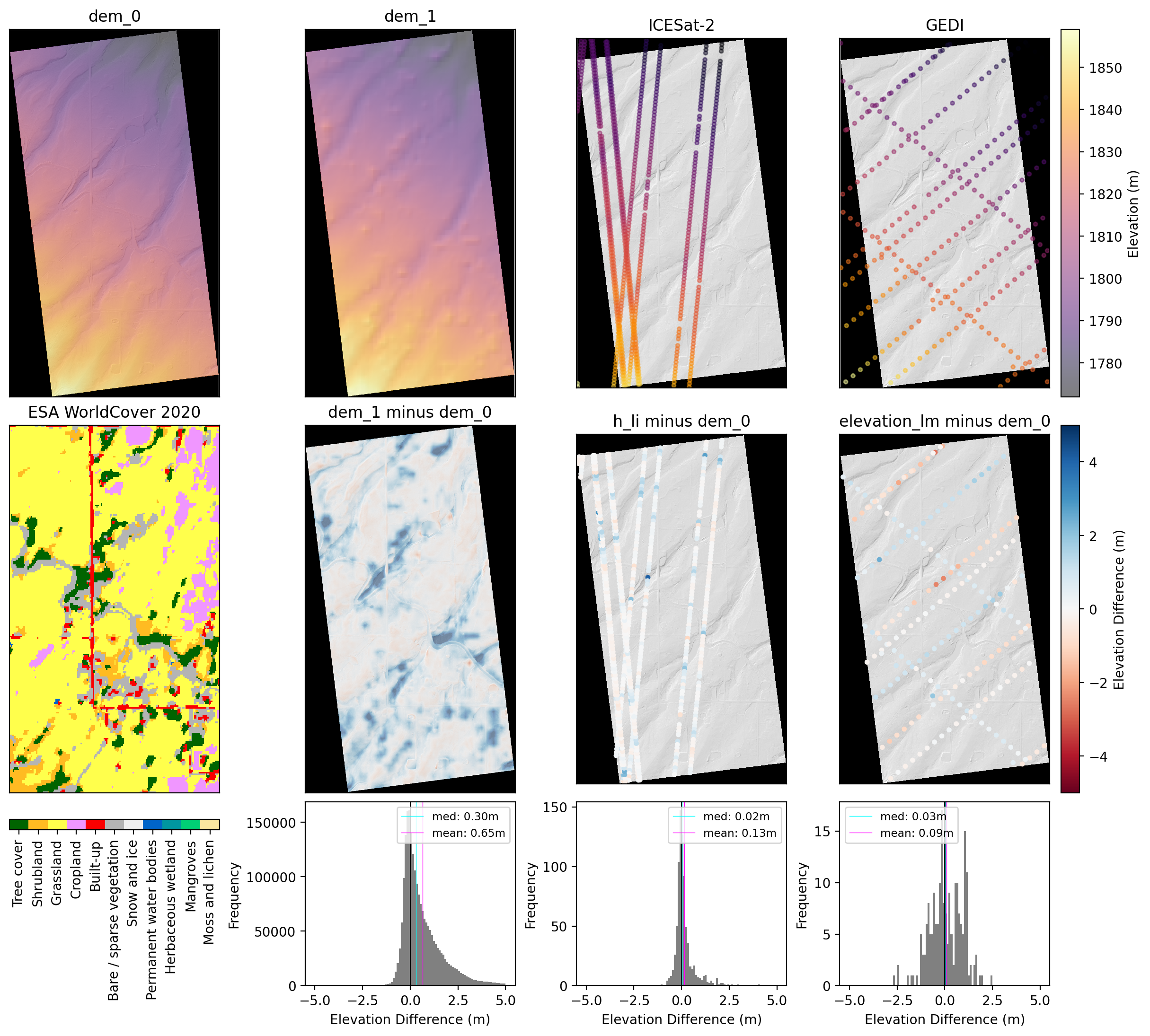
Main Elevation Comparison Panel#
‘coincident’ supports a main compare_dems function that allows you to compare multiple DEMs and altimetry points in a single panel. This function dynamically adjusts based on the number of datasets provided.
Note
compare_dems assumes that all DEMs are in the same coordinate reference system (CRS) and aligned. It also assumes that each DEM has an ‘elevation’ variable. If add_hillshade=True, it assumes the first DEM passed has a ‘hillshade’ variable, where the ‘hillshade’ variable can be calculated with coincident.plot.create_hillshade as seen below. A minimum of two DEMs must be provided and a maximum of 5 total datasets (datasets being DEMs and GeoDataFrames of altimetry points) can be provided.
# list of DEMs to compare, where the first DEM in the list is the 'source' DEM
dem_list = [ds_lidar, ds_cop_r]
# dictionary of GeoDataFrames with altimetry points to compare
# where the key is the name/plot title of the dataset and the value is a tuple of the respective
# GeoDataFrame and the column name of the elevation values of interest
dicts_gds = {"ICESat-2": (data_is2, "h_li"), "GEDI": (data_gedi, "elevation_lm")}

axd = coincident.plot.compare_dems(
    dem_list,
    dicts_gds,
    # ds_wc=ds_wc,
    add_hillshade=True,
    diff_clim=(-5, 5),  # difference colormap limits
)
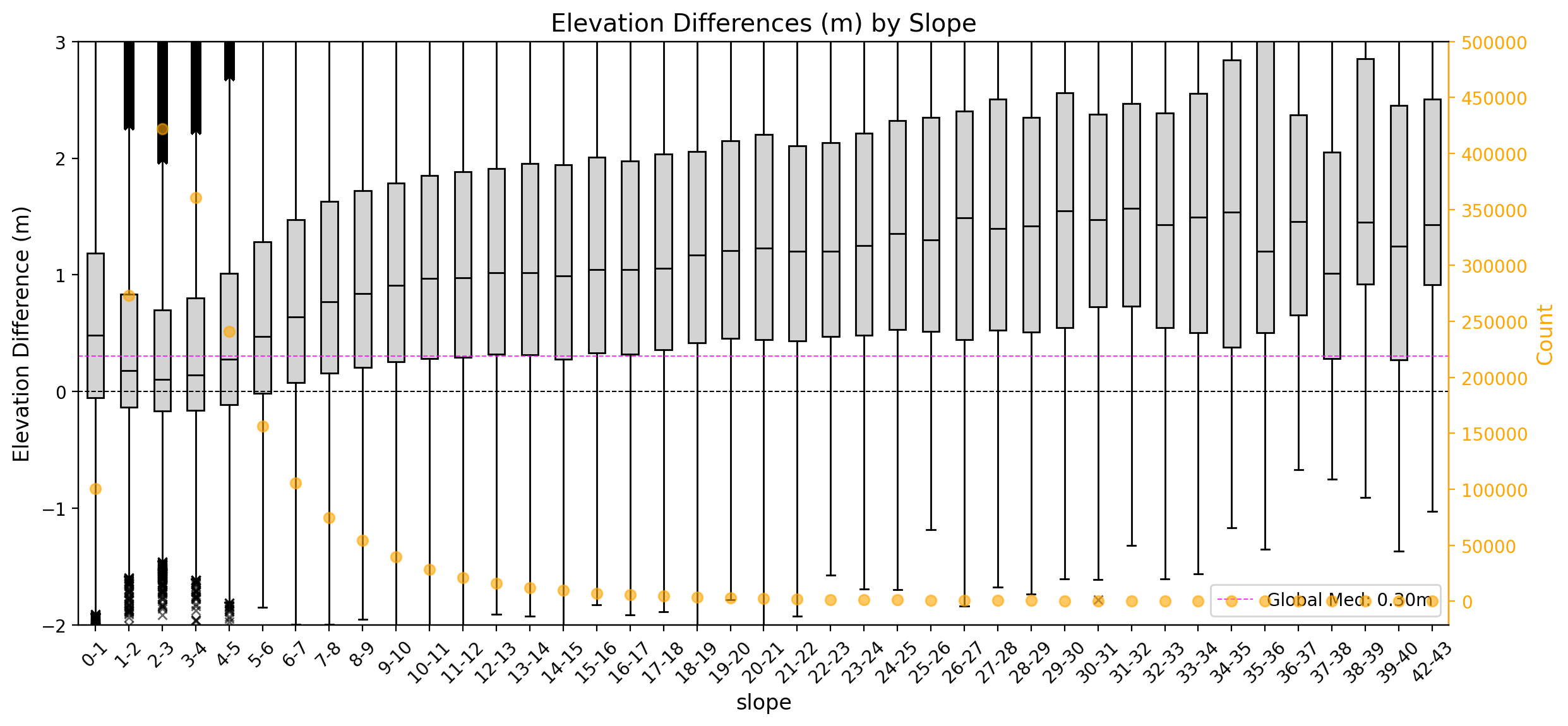
Dynamic Elevation Difference Boxplots Based on Terrain Variables (slope, elevation, aspect)#
coincident allows users to dynamically plot elevation differences based on grouped data such as slope values. In these functions (that are wrappers for the generalized coincident.plot.boxplot_terrain_diff function), the user provides a reference DEM and one other DEM or GeoDataFrame with elevation values to compare to. These function assumes that the reference DEM has the respective terrain variable (slope, aspect, etc.) of interest.
Note
Boxplots will only be generated with groups of value counts greater than 30. Dynamic ylims will be fit to the IQRs of the boxplots.
# THese routines assume rectilinear data, so we first convert to UTM
crs_utm = ds_lidar.rio.estimate_utm_crs()
ds_lidar_utm = ds_lidar.rio.reproject(crs_utm)
ds_cop_utm = ds_cop_r.rio.reproject(crs_utm)
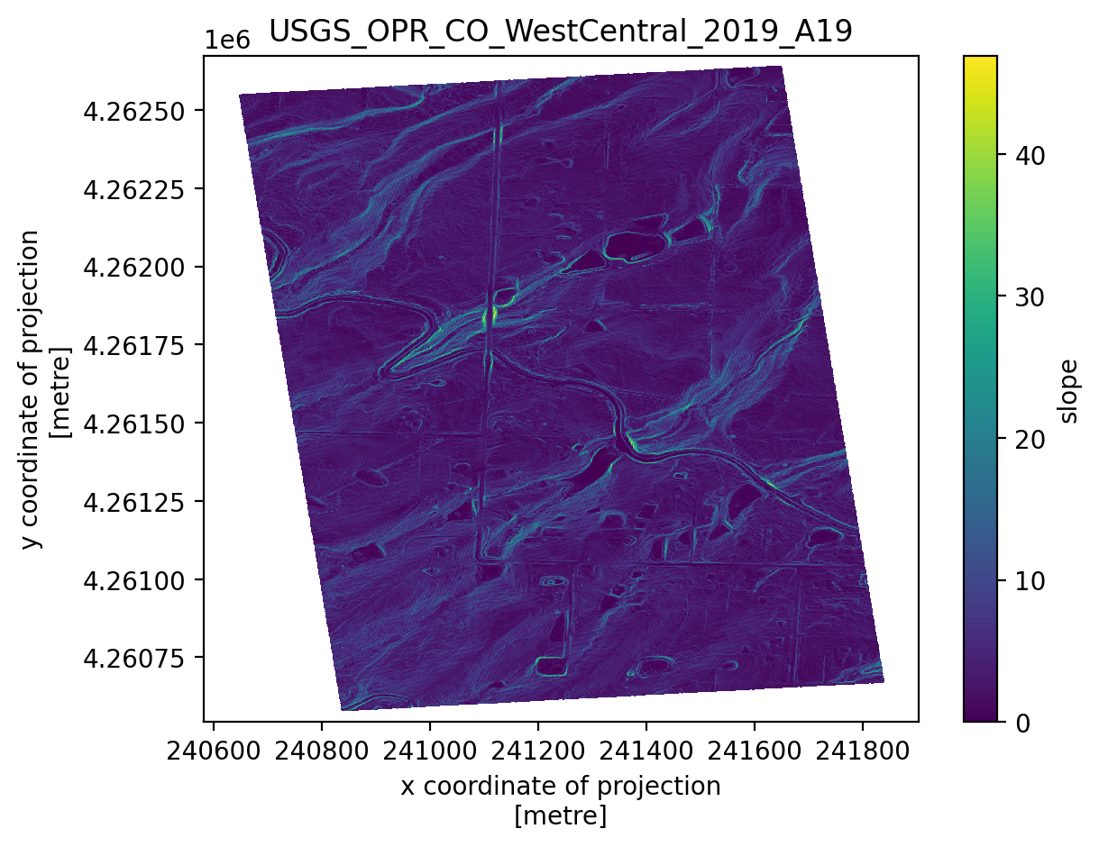
slope = xdem.terrain.slope(
    ds_lidar_utm.elevation.values, resolution=ds_lidar_utm.rio.resolution()[0]
)
ds_lidar_utm["slope"] = (("y", "x"), np.squeeze(slope))
_, ax = plt.subplots()
ds_lidar_utm.slope.plot.imshow(ax=ax)
ax.set_title("USGS_OPR_CO_WestCentral_2019_A19");
ax_boxplot_dems = coincident.plot.boxplot_slope([ds_lidar_utm, ds_cop_utm])
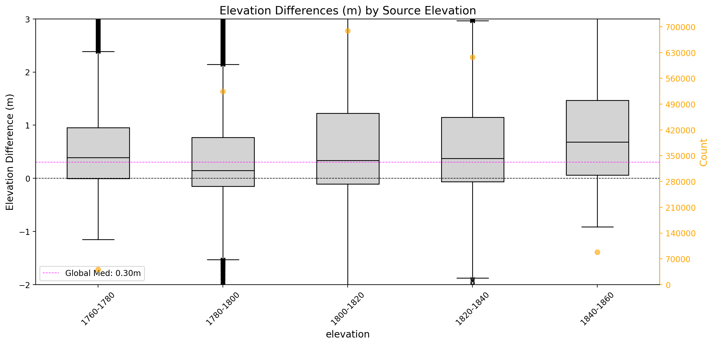
# we also support elevation differences based on elevation bins
# grouped on the reference DEM's elevation values
ax_elev = coincident.plot.boxplot_elevation(
    [ds_lidar_utm, ds_cop_utm], elevation_bins=np.arange(1700, 2000, 20)
)
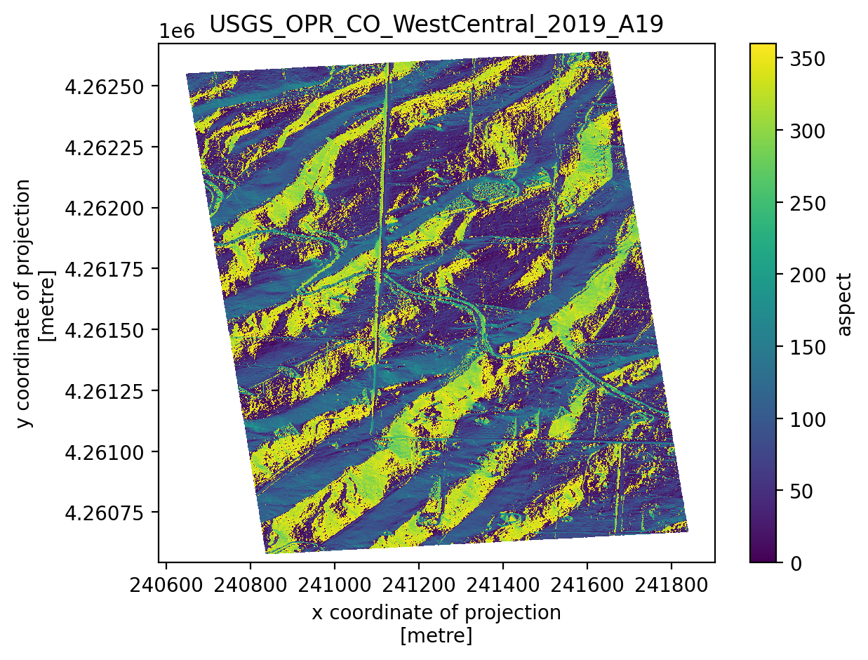
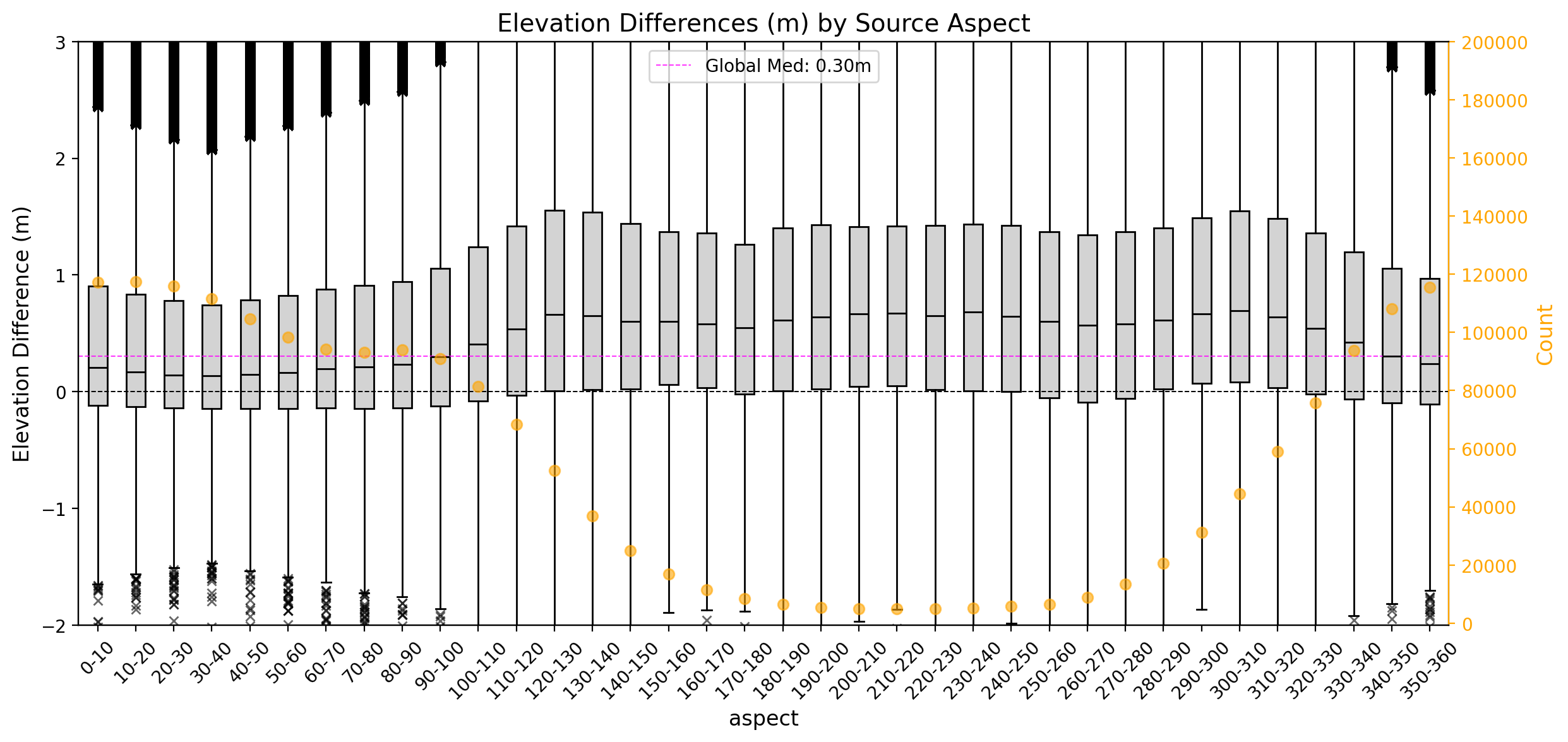
# lastly for the boxplots, let's look at aspect
aspect = xdem.terrain.aspect(ds_lidar_utm.elevation.values)
ds_lidar_utm["aspect"] = (("y", "x"), np.squeeze(aspect))
_, ax = plt.subplots()
ds_lidar_utm.aspect.plot.imshow(ax=ax)
ax.set_title("USGS_OPR_CO_WestCentral_2019_A19");
ax_aspect = coincident.plot.boxplot_aspect([ds_lidar_utm, ds_cop_utm])
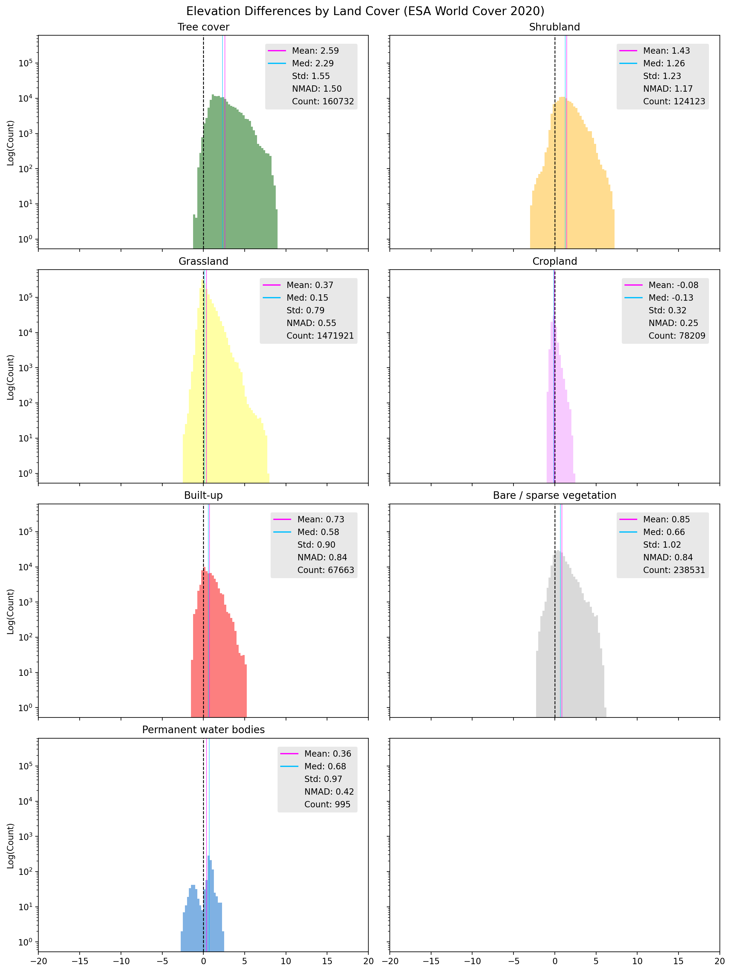
Histograms of Elevation Differences over Land Cover#
Plot elevation differences between DEMs or point data, grouped by ESA World Cover 2020 land cover class
Note
Histograms will only be generated with groups of value counts greater than a user-defined threshold (default is 30).
ax_lulc_cop30 = coincident.plot.hist_esa([ds_lidar, ds_cop_r])