Contextual data#
Once you’ve identified areas of interest where multiple datasets intersect, you can pull additional data to provide further context. For example:
landcover
global elevation data
import coincident
import matplotlib.pyplot as plt
import xarray as xr
import numpy as np
import rasterio
from shapely.geometry import box
import geopandas as gpd
/home/docs/checkouts/readthedocs.org/user_builds/coincident/checkouts/stable/src/coincident/io/download.py:25: TqdmExperimentalWarning: Using `tqdm.autonotebook.tqdm` in notebook mode. Use `tqdm.tqdm` instead to force console mode (e.g. in jupyter console)
  from tqdm.autonotebook import tqdm
%matplotlib inline
# %config InlineBackend.figure_format = 'retina'
Identify a primary dataset#
Start by loading a full resolution polygon of a 3DEP LiDAR workunit which has a known start_datetime and end_datatime:
workunit = "CO_WestCentral_2019"
df_wesm = coincident.search.wesm.read_wesm_csv()
gf_lidar = coincident.search.wesm.load_by_fid(
    df_wesm[df_wesm.workunit == workunit].index
)

gf_lidar
| workunit | workunit_id | project | project_id | start_datetime | end_datetime | ql | spec | p_method | dem_gsd_meters | ... | seamless_category | seamless_reason | lpc_link | sourcedem_link | metadata_link | geometry | collection | datetime | dayofyear | duration | |
|---|---|---|---|---|---|---|---|---|---|---|---|---|---|---|---|---|---|---|---|---|---|
| 0 | CO_WestCentral_2019 | 175984 | CO_WestCentral_2019_A19 | 175987 | 2019-08-21 | 2019-09-19 | QL 2 | USGS Lidar Base Specification 1.3 | linear-mode lidar | 1.0 | ... | Meets | Meets 3DEP seamless DEM requirements | https://rockyweb.usgs.gov/vdelivery/Datasets/S... | https://prd-tnm.s3.amazonaws.com/index.html?pr... | https://prd-tnm.s3.amazonaws.com/index.html?pr... | MULTIPOLYGON (((-106.13571 38.4146, -106.1702 ... | 3DEP | 2019-09-04 12:00:00 | 247 | 29 |
1 rows × 33 columns
search_aoi = gf_lidar.simplify(0.01)
Search for coincident contextual data#
Coincident provides two convenience functions to load datasets resulting from a given search.
gf_wc = coincident.search.search(
    dataset="worldcover",
    intersects=search_aoi,
    # worldcover is just 2020 an 2021, so pick one
    datetime=["2020"],
)
gf_wc.iloc[0]  # NOTE: asset key = 'map' (depends on upstream STAC catalog)
type                                                                        Feature
stac_version                                                                  1.1.0
stac_extensions                   [https://stac-extensions.github.io/projection/...
id                                             ESA_WorldCover_10m_2020_v100_N39W108
proj:code                                                                 EPSG:4326
esa_worldcover:product_version                                                1.0.0
links                             [{'href': 'https://planetarycomputer.microsoft...
assets                            {'map': {'href': 'https://ai4edataeuwest.blob....
collection                                                           esa-worldcover
datetime                                                                        NaT
start_datetime                                            2020-01-01 00:00:00+00:00
end_datetime                                              2020-12-31 23:59:59+00:00
description                                ESA WorldCover product at 10m resolution
created                                            2023-04-06 15:30:59.849000+00:00
mission                                                      sentinel-1, sentinel-2
platform                          sentinel-1a, sentinel-1b, sentinel-2a, sentine...
grid:code                                                     ESAWORLDCOVER-N39W108
instruments                                                            [c-sar, msi]
esa_worldcover:product_tile                                                 N39W108
bbox                              {'xmin': -108.0, 'ymin': 39.0, 'xmax': -105.0,...
geometry                          POLYGON ((-108 42, -108 39, -105 39, -105 42, ...
dayofyear                                                                       NaN
Name: 0, dtype: object
gf_cop30 = coincident.search.search(
    dataset="cop30",
    intersects=search_aoi,
)
gf_cop30.iloc[0].assets  # NOTE: asset key = 'data'
{'data': {'href': 'https://elevationeuwest.blob.core.windows.net/copernicus-dem/COP30_hh/Copernicus_DSM_COG_10_N39_00_W108_00_DEM.tif',
  'title': 'N39_00_W108_00',
  'type': 'image/tiff; application=geotiff; profile=cloud-optimized',
  'roles': array(['data'], dtype=object)},
 'tilejson': {'href': 'https://planetarycomputer.microsoft.com/api/data/v1/item/tilejson.json?collection=cop-dem-glo-30&item=Copernicus_DSM_COG_10_N39_00_W108_00_DEM&assets=data&colormap_name=terrain&rescale=-1000%2C4000&format=png',
  'title': 'TileJSON with default rendering',
  'type': 'application/json',
  'roles': array(['tiles'], dtype=object)},
 'rendered_preview': {'href': 'https://planetarycomputer.microsoft.com/api/data/v1/item/preview.png?collection=cop-dem-glo-30&item=Copernicus_DSM_COG_10_N39_00_W108_00_DEM&assets=data&colormap_name=terrain&rescale=-1000%2C4000&format=png',
  'title': 'Rendered preview',
  'type': 'image/png',
  'roles': array(['overview'], dtype=object),
  'rel': 'preview'}}
STAC search results to datacube#
If the results have STAC-formatted metadata. We can take advantage of the excellent odc.stac tool to load datacubes. Please refer to odc.stac documentation for all the configuration options (e.g. setting resolution our output CRS, etc.)
By default this uses the dask parallel computing library to intelligently load only metadata initially and defer reading values until computations or visualizations are performed.
Copernicus DEM#
ds = coincident.io.xarray.to_dataset(
    gf_cop30,
    aoi=search_aoi,
    # chunks=dict(x=2048, y=2048), # manual chunks
    # resolution=0.00081,  # ~90m
    resolution=0.00162,
    mask=True,
)
# By default, these are dask arrays, data is not read until needed for computations or plots
ds
<xarray.Dataset> Size: 4MB
Dimensions:      (latitude: 769, longitude: 1144, time: 1)
Coordinates:
  * latitude     (latitude) float64 6kB 39.39 39.39 39.39 ... 38.15 38.15 38.14
  * longitude    (longitude) float64 9kB -108.0 -108.0 -108.0 ... -106.1 -106.1
  * time         (time) datetime64[us] 8B 2021-04-22
    spatial_ref  int64 8B 0
Data variables:
data (time, latitude, longitude) float32 4MB dask.array<chunksize=(1, 769, 1144), meta=np.ndarray># The CRS is taken to be whatever is stored in STAC metadata
ds.rio.crs.to_epsg()
4326
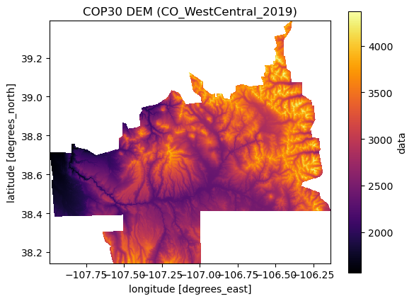
# Convert to 2D DataArray and load into memory
da_cop = ds["data"].squeeze().compute()
coincident.plot.plot_dem(da_cop, title="COP30 DEM (CO_WestCentral_2019)");
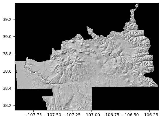
Hillshades#
# We have a convenience function to create a hillshade with GDAL:
da_hillshade = coincident.io.gdal.gdaldem(da_cop, subcommand="hillshade")
da_hillshade.plot.imshow(cmap="gray", alpha=1.0, add_colorbar=False, add_labels=False);
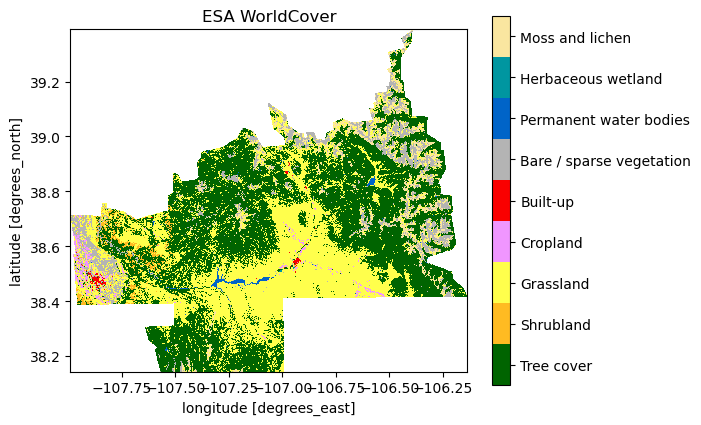
ESA Worldcover#
# Same with LandCover
dswc = coincident.io.xarray.to_dataset(
    gf_wc,
    bands=["map"],  # NOTE: STAC Asset key is 'map' rather than 'data'
    # Customize the area of interest and resolution if desired:
    # aoi=search_aoi,
    # mask=True,
    # resolution=0.00027, #~30m
    # resolution=0.00081,  # ~90m
    # Or match the low resolution elevation data:
    like=da_cop,
)
dswc
<xarray.Dataset> Size: 895kB
Dimensions:      (latitude: 769, longitude: 1144, time: 1)
Coordinates:
  * latitude     (latitude) float64 6kB 39.39 39.39 39.39 ... 38.15 38.15 38.14
  * longitude    (longitude) float64 9kB -108.0 -108.0 -108.0 ... -106.1 -106.1
  * time         (time) datetime64[us] 8B 2020-01-01
    spatial_ref  int32 4B 4326
Data variables:
map (time, latitude, longitude) uint8 880kB dask.array<chunksize=(1, 769, 1144), meta=np.ndarray># Unfortunately due to floating point precision issues, we need to explicitly match coordinate values
da_wc = dswc["map"].squeeze().compute().assign_coords(da_cop.coords)
da_wc = da_wc.where(da_cop.notnull())
# For landcover there is a convenicence function for a nice categorical colormap
ax = coincident.plot.plot_esa_worldcover(da_wc)
ax.set_title("ESA WorldCover");
Load gridded elevation in a consistent CRS#
coincident also has a convenience function for loading gridded elevation datasets in a consistent CRS. In order to facilitate comparison with modern altimetry datasets (ICESat-2, GEDI), we convert elevation data on-the-fly to EPSG:7912. 3D Coordinate Reference Frames are a complex topic, so please see this resource for more detail on how these conversions are done: https://uw-cryo.github.io/3D_CRS_Transformation_Resources/
Note
Currently gridded DEMs are retrieved from OpenTopography hosted in AWS us-west-2.
Warning
The output of load_dem_7912() uses the native resolution and grid of the input dataset, and data is immediately read into memory. So this method is better suited to small AOIs.
# Start with a small AOI:
aoi = gpd.GeoDataFrame(
    geometry=[box(-106.812163, 38.40825, -106.396812, 39.049796)], crs="EPSG:4326"
)
da_cop = coincident.io.xarray.load_dem_7912("cop30", aoi=aoi)
# NASA DEM and COP30 DEM are both 30m but will not necessarily have same coordinates!
da_nasa = coincident.io.xarray.load_dem_7912("nasadem", aoi=aoi)
# We check that coordinates are sufficiently close before force-alignment.
# If sufficiently different, it would be better to use rioxarray.reproject_match!
xr.testing.assert_allclose(da_cop.x, da_nasa.x)  # rtol=1e-05, atol=1e-08 defaults
xr.testing.assert_allclose(da_cop.y, da_nasa.y)
da_nasa = da_nasa.assign_coords(x=da_cop.x, y=da_cop.y)
diff = da_cop - da_nasa
median = diff.median()
mean = diff.mean()
std = diff.std()

fig = plt.figure(layout="constrained", figsize=(4, 8))  # figsize=(8.5, 11)
ax = fig.add_gridspec(top=0.75).subplots()
ax_histx = ax.inset_axes([0, -0.35, 1, 0.25])
axes = [ax, ax_histx]
diff.plot.imshow(
    ax=axes[0], robust=True, add_colorbar=False
)  # , cbar_kwargs={'label': ""})
n, bins, ax = diff.plot.hist(ax=axes[1], bins=100, range=(-20, 20), color="gray")
approx_mode = bins[np.argmax(n)]
axes[0].set_title("COP30 - NASADEM")
axes[0].set_aspect(aspect=1 / np.cos(np.deg2rad(38.7)))
axes[1].axvline(0, color="k")
axes[1].axvline(median, label=f"median={median:.2f}", color="cyan", lw=1)
axes[1].axvline(mean, label=f"mode={mean:.2f}", color="magenta", lw=1)
axes[1].axvline(approx_mode, label=f"mode={approx_mode:.2f}", color="yellow", lw=1)
axes[1].set_xlabel("Elevation difference (m)")
axes[1].legend()
axes[1].set_title("");
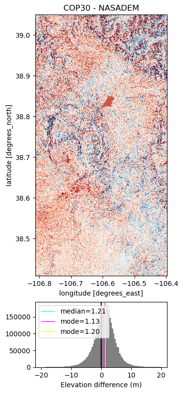
Note
We see that COP30 elevation values are approximately 1m greater than NASADEM values for this area. Such a difference is within the stated accuracies of each gridded dataset, and also COP30 is derived from X-band TanDEM-X observations with nominal time of 2021-04-22 whereas NASADEM is primarily based on C-band SRTM collected 2000-02-20.
# Load 3DEP 10m data
da_3dep = coincident.io.xarray.load_dem_7912("3dep", aoi=aoi)
# To compare to 3dep, we refine cop30 from 30m to 10m using bilinear resampling
da_cop_r = da_cop.rio.reproject_match(
    da_3dep, resampling=rasterio.enums.Resampling.bilinear
)
da_nasa_r = da_nasa.rio.reproject_match(
    da_3dep, resampling=rasterio.enums.Resampling.bilinear
).compute()
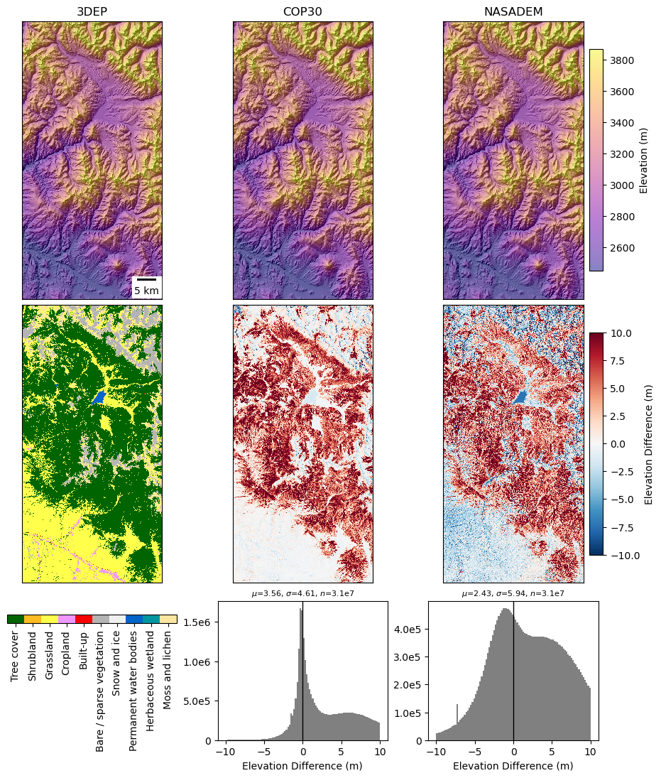
Comparing multiple DEMs#
coincident has a convenience function for comparing multiple DEMs. It is your responsibility to ensure the DEMs are on the same grid and have the same CRS!
ax = coincident.plot.compare_dems(
    dem_dict={
        "3DEP": da_3dep,
        "COP30": da_cop_r,
        "NASADEM": da_nasa_r,
    },
    downsample_factor=4,  # for low-RAM, coarsen arrays shown with imshow
    add_hillshade=True,
)